Understanding Cumulative Distribution Functions (CDF) and Their Empirical Estimation#
Introduction to CDFs#
Before diving into empirical distributions, it’s essential to understand what a cumulative distribution function represents and why it’s useful in statistical analysis. A CDF helps us understand the complete probability distribution of a random variable by showing the probability of the variable being less than or equal to any given value.
CDF Definition and Intuition#
The CDF \(F_X(x)\) of a random variable \(X\) gives the probability that \(X\) is less than or equal to \(x\):
\(F_X(x) = P(X \leq x)\)
To build intuition:
If we’re measuring heights in a population, \(F_X(170)\) would tell us the proportion of people who are 170 cm or shorter
For test scores, \(F_X(80)\) would represent the fraction of students scoring 80 or below
In reliability analysis, \(F_X(t)\) might represent the probability of a component failing by time \(t\)
CDF for Discrete Random Variables#
For a discrete random variable \(X\) with probability mass function (PMF) \(p_X(x)\), the CDF is the cumulative sum of the probabilities up to \(x\):
\(F_X(x) = \sum_{x_i \leq x} p_X(x_i)\)
Example: Rolling a Die#
Consider rolling a fair six-sided die:
\(P(X \leq 3) = P(X = 1) + P(X = 2) + P(X = 3) = \frac{1}{6} + \frac{1}{6} + \frac{1}{6} = \frac{1}{2}\)
The CDF would jump by \(\frac{1}{6}\) at each value from 1 to 6
CDF for Continuous Random Variables#
For a continuous random variable \(X\) with probability density function (PDF) \(f_X(x)\), the CDF is the integral of the PDF from \(-\infty\) to \(x\):
\(F_X(x) = \int_{-\infty}^{x} f_X(t) \, dt\)
Example: Normal Distribution#
For a standard normal distribution:
The CDF at \(x = 0\) is 0.5, meaning 50% of the data lies below zero
The CDF at \(x = 1\) is approximately 0.84, indicating about 84% of the data lies below 1
Properties of CDF#
The CDF has several important properties that make it useful for statistical analysis:
Non-decreasing:
The CDF is always non-decreasing: \(F_X(x) \leq F_X(y)\) for \(x \leq y\)
This makes intuitive sense as accumulating probabilities can’t decrease
Limits:
\(\lim_{x \to -\infty} F_X(x) = 0\): The probability of getting an infinitely small value is zero
\(\lim_{x \to \infty} F_X(x) = 1\): The probability of getting any value is 1 (certainty)
Right-continuity:
\(\lim_{\epsilon \to 0^+} F_X(x + \epsilon) = F_X(x)\)
This ensures smooth behavior when approaching values from the right
Particularly important for discrete distributions where jumps occur
Range:
\(0 \leq F_X(x) \leq 1\) for all \(x\)
This follows from the basic properties of probability
Empirical CDF (ECDF)#
The empirical CDF is a practical tool for estimating the true CDF when we only have sample data. Given a sample \(X_1, X_2, \dots, X_n\), the ECDF \(\hat{F}_n(x)\) is defined as:
\(\hat{F}_n(x) = \frac{1}{n} \sum_{i=1}^{n} \mathbb{I}(X_i \leq x)\)
Where:
\(\mathbb{I}(X_i \leq x)\) is the indicator function
\(n\) is the sample size
\(\hat{F}_n(x)\) represents the proportion of data points ≤ \(x\)
Example: Computing ECDF#
For the dataset {1, 2, 2, 3, 4, 4, 5}:
\(\hat{F}_n(2) = \frac{3}{7}\) (3 values ≤ 2)
\(\hat{F}_n(4) = \frac{6}{7}\) (6 values ≤ 4)
The function jumps by \(\frac{1}{7}\) at each unique value
Practical Applications of ECDF#
Non-parametric Estimation
Provides distribution estimates without assuming a specific form
Useful when the underlying distribution is unknown
More robust than parametric methods
Goodness-of-fit Testing
Kolmogorov-Smirnov test compares ECDF to theoretical CDF
Helps validate distribution assumptions
Example: Testing if data follows a normal distribution
Quantile Estimation
Find sample percentiles directly from ECDF
Median: Value where ECDF = 0.5
Quartiles: Values where ECDF = 0.25, 0.75
Anomaly Detection
Identify outliers using ECDF percentiles
Points in extreme tails (e.g., ECDF > 0.99) might be anomalies
More robust than parametric methods
import numpy as np
import matplotlib.pyplot as plt

plt.style.use('dark_background')
np.random.seed(47)
# Generate data
mean = 0
std = 2
sample_size = 500
sample = np.random.normal(loc=mean, scale=std, size=sample_size)
# Define support range (empirical)
support = (min(sample) - 0.5, max(sample) + 0.5)

# Number of points to calculate the relative frequency for
num_points = 20
points = np.linspace(support[0], support[1], num_points)

# Calculate relative frequencies
cumulative_reqlative_frequencies = []
for point in points:
    cumulative_reqlative_frequencies.append(
        (sample <= point).sum() / sample_size
    )
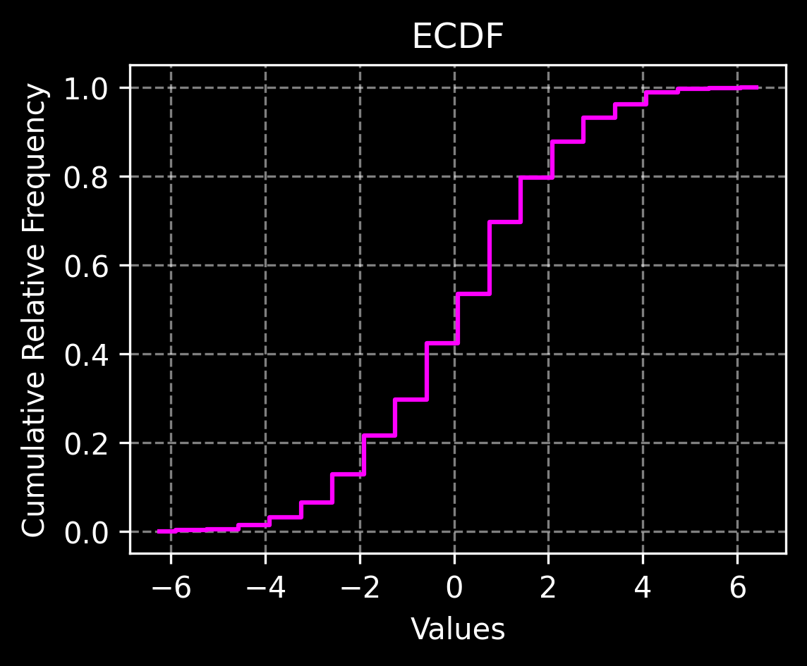
# Plot the cumulative relative frequencies vs points
plt.figure(figsize=(4, 3), dpi=300)
plt.step(points, cumulative_reqlative_frequencies,
         where='mid', color='magenta')
plt.xlabel('Values')
plt.ylabel('Cumulative Relative Frequency')
plt.title('ECDF')
plt.grid(True, alpha=0.5, linestyle='--')
plt.show()