PCA-based Reconstruction#
PCA using the Correlation Matrix
Standardization: \( x_{\text{standardized}}^{(i)} = \frac{x^{(i)} - \mu^{(i)}}{\sigma^{(i)}} \) where:
\(\mu^{(i)}\): Mean of \(i\)-th feature column
\(\sigma^{(i)}\): Standard deviation of \(i\)-th feature column
\(x^{(i)}\): \(i\)-th feature column
\(x_{\text{standardized}}^{(i)}\): Standardized \(i\)-th feature column (zero mean, unit variance)
Sample Correlation Matrix: \( R = \frac{1}{n-1} X_{\text{standardized}}^T X_{\text{standardized}} \) where:
\(R\): Correlation matrix of size (features × features)
\(n\): Number of samples
\(X_{\text{standardized}}\): Matrix of all standardized columns (samples × features)
Eigenvalue Decomposition: \( R = V \Lambda V^T \) where:
\(V\): Matrix of eigenvectors (principal components) of size (features × features)
\(\Lambda\): Diagonal matrix of eigenvalues (variances along principal components)
\(V^T\): Transpose of eigenvector matrix
Projection: \( Z = X_{\text{standardized}} V \) where:
\(Z\): Projected data in principal component space (samples × features)
\(V\): Principal component directions
Reconstruction: \( X_{\text{reconstructed}} = Z V^T D + M \) where:
\(X_{\text{reconstructed}}\): Data reconstructed in original space
\(D\): Diagonal matrix of original standard deviations (features × features)
\(M\): Matrix of means (samples × features), where each row is the mean vector repeated
Key Points:
Use \(n-1\) for unbiased estimation in the correlation matrix (Bessel’s Correction)
Each feature column \(x^{(i)}\) is standardized independently
Eigenvalues in \(\Lambda\) represent the variance explained by each principal component
\(V\) columns are sorted by decreasing eigenvalues (most important components first)
Perfect reconstruction is possible using all components, lossy when using fewer
\(D\) is a diagonal matrix of standard deviations (features × features)
\(M\) is mean matrix created by repeating mean vector for each sample (samples × features)
import numpy as np
import matplotlib.pyplot as plt
from matplotlib.lines import Line2D

# Data Generation
np.random.seed(47)
plt.style.use('dark_background')
mean = np.array([5, 10])
cov = np.array([[10, 3], [3, 1]])
n = 100
X = np.random.multivariate_normal(mean, cov, size=n)

# Adding anomalies
anomalies = np.array([[5, 12], [-2.5, 2], [10, 14]])
X = np.vstack([X, anomalies])
n = X.shape[0]
# Standardizing the data
X_mean = np.mean(X, axis=0)
X_std = np.std(X, axis=0)
X_standardized = (X - X_mean) / X_std

# Covariance matrix and PCA
R = X_standardized.T @ X_standardized / (n - 1)
eigenvalues, eigenvectors = np.linalg.eigh(R)
sorted_indices = np.argsort(eigenvalues)[::-1]
eigenvalues = eigenvalues[sorted_indices]
eigenvectors = eigenvectors[:, sorted_indices]

# Projecting and reconstructing
Z = X_standardized @ eigenvectors[:, :1]
D = np.diag(X_std)
X_reconstructed = (
    Z @ eigenvectors[:, :1].T @ D + X_mean
)

# Reconstruction errors
reconstruction_errors = np.linalg.norm(X - X_reconstructed, ord=2, axis=1)
threshold = np.percentile(reconstruction_errors, 95)  # Threshold for anomaly detection (95th percentile)

# Step 6: Print original and reconstructed data samples
print("\nOriginal Data (first 5 samples):\n", X[:5])
print("\nReconstructed Data (first 5 samples):\n", X_reconstructed[:5])
Original Data (first 5 samples):
 [[ 7.56602935 11.19005407]
 [ 2.02233349  9.30102911]
 [ 8.17635236 11.53044291]
 [ 8.12921555 11.20800311]
 [ 5.98339063 10.11031892]]

Reconstructed Data (first 5 samples):
 [[ 7.6611491  11.14965863]
 [ 2.66524339  9.02799825]
 [ 8.36706998 11.44944899]
 [ 7.96387464 11.27822006]
 [ 5.59859543 10.27373369]]
# Visualizations
plt.figure(figsize=(8, 6), dpi=300)
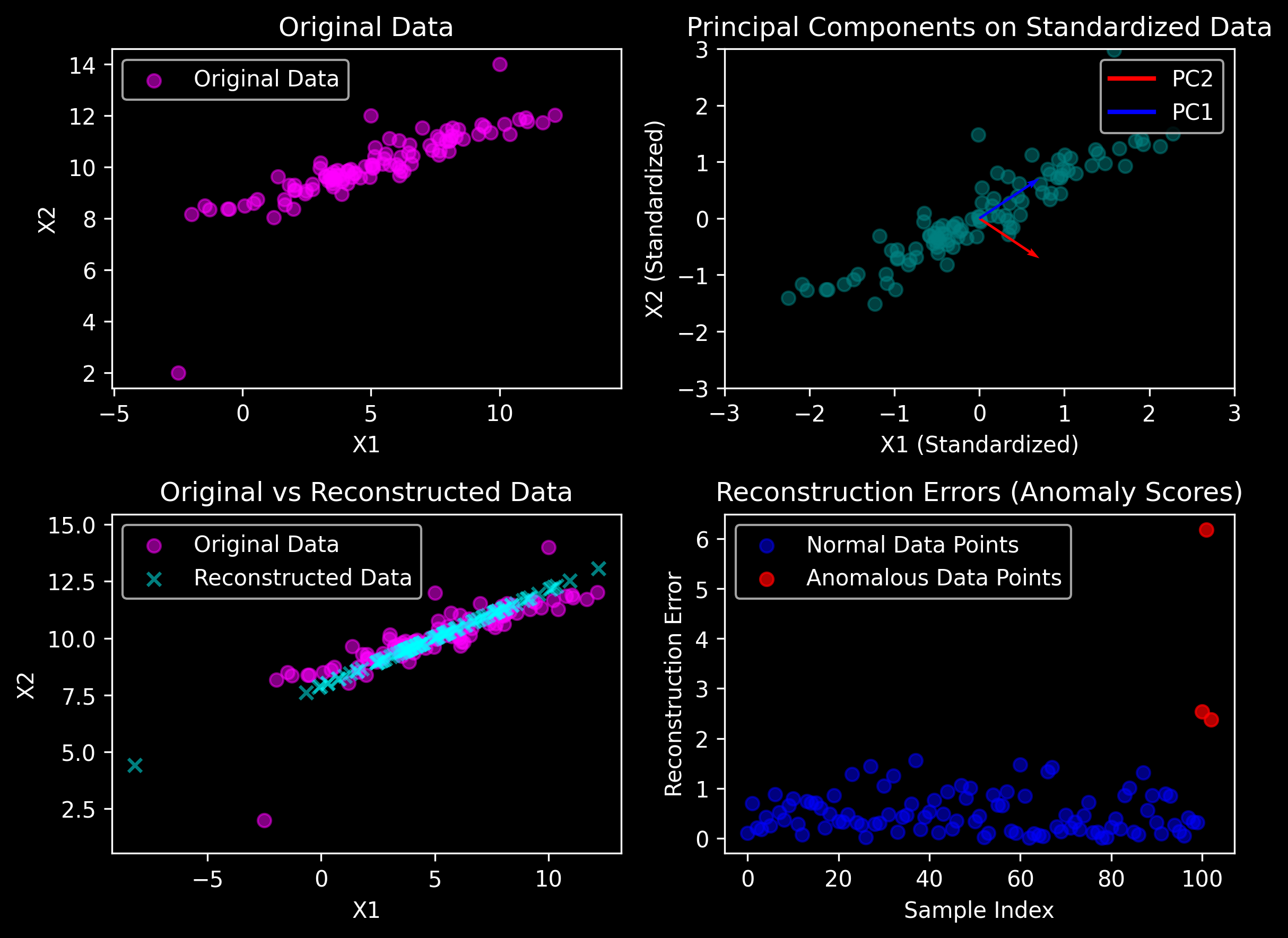
# Plot-1: Original Data
plt.subplot(2, 2, 1)
plt.scatter(X[:, 0], X[:, 1], alpha=0.5, label="Original Data", color='magenta')
plt.title("Original Data")
plt.xlabel("X1")
plt.ylabel("X2")
plt.axis("equal")
plt.legend()
# Plot-2: Principal Components on Standardized Data
plt.subplot(2, 2, 2)
plt.scatter(X_standardized[:, 0], X_standardized[:, 1], alpha=0.5, label="Standardized Data", color='teal')
origin = np.zeros((2, 2)) # Two origins, one for each eigenvector
plt.quiver(
origin[:, 0], origin[:, 1], # Origin points
eigenvectors[:, 0], eigenvectors[:, 1], # Eigenvector components
angles='xy', scale_units='xy', scale=1, color=['r', 'b'], width=0.005
)
plt.xlim(-3, 3)
plt.ylim(-3, 3)
plt.title("Principal Components on Standardized Data")
plt.xlabel("X1 (Standardized)")
plt.ylabel("X2 (Standardized)")
# Create custom legend handles for arrows
legend_elements = [Line2D([0], [0], color='r', lw=2, label='PC2'),
Line2D([0], [0], color='b', lw=2, label='PC1')]
plt.legend(handles=legend_elements)
# Plot-3: Original vs Reconstructed Data
plt.subplot(2, 2, 3)
plt.scatter(X[:, 0], X[:, 1], alpha=0.5, label="Original Data", color='magenta')
plt.scatter(X_reconstructed[:, 0], X_reconstructed[:, 1], alpha=0.5, label="Reconstructed Data", marker='x', color='cyan')
plt.title("Original vs Reconstructed Data")
plt.xlabel("X1")
plt.ylabel("X2")
plt.axis("equal")
plt.legend()
# Plot-4: Reconstruction Errors and Highlight Anomalies
plt.subplot(2, 2, 4)
plt.scatter(np.arange(len(reconstruction_errors))[:-3], reconstruction_errors[:-3],
color='blue', alpha=0.5, label="Normal Data Points")
plt.scatter(np.arange(len(reconstruction_errors))[-3:], reconstruction_errors[-3:],
color='red', alpha=0.7, label="Anomalous Data Points")
plt.title("Reconstruction Errors (Anomaly Scores)")
plt.xlabel("Sample Index")
plt.ylabel("Reconstruction Error")
plt.legend()
plt.tight_layout()
plt.show()