Gaussian Error Linear Unit (GeLU)#
Definition and Formula#
GeLU activation function is defined as:
\(\text{GeLU}(x) = x \cdot \Phi(x)\)
where \(\Phi(x)\) is the cumulative distribution function (CDF) of the standard normal distribution:
\(\Phi(x) = \frac{1}{2}[1 + \text{erf}(\frac{x}{\sqrt{2}})]\)
Practical Approximation#
For computational efficiency, GeLU can be approximated as:
\(\text{GeLU}(x) \approx 0.5x(1 + \tanh[\sqrt{2/\pi}(x + 0.044715x^3)])\)
Intuition Behind GeLU#
In GeLU, the output is \(x \Phi(x)\), where \(\Phi(x)\) is the cumulative distribution function (CDF) of the standard normal distribution. This combines \(x\) with a probabilistic weighting based on its magnitude and sign, as determined by the CDF.
Key Interactions#
Large positive \(x\)#
\(\Phi(x) \approx 1\), so \(x\) is kept almost as-is
These values are important and should be retained
Behavior similar to ReLU in this region
Small positive \(x\)#
\(\Phi(x) < 1\), so \(x\) is scaled down
These values are less critical but still contribute
Provides smooth transition unlike ReLU
Large negative \(x\)#
\(\Phi(x) \approx 0\), so \(x\) is suppressed
Reduces large negative contributions
Helps prevent destabilizing large negative summations
Near-zero \(x\)#
Function smoothly transitions
Ensures differentiability
Avoids sharp cuts like ReLU
Note: GeLU is a deterministic function. There is no random sampling happening. The key idea is that input values are modulated according to their magnitude and sign, using the CDF of the standard normal distribution.
Comparison with Common Activation Functions#
ReLU#
\(\text{ReLU}(x) = \max(0, x)\)
Most commonly used activation function
Zero output for negative inputs
Linear for positive inputs
Non-differentiable at \(x = 0\)
Leaky ReLU#
\(\text{Leaky ReLU}(x) = \max(\alpha x, x)\), where \(\alpha\) is typically 0.01
Modified version of ReLU
Small positive slope for negative inputs
Still non-differentiable at \(x = 0\)
Fixed slope parameter \(\alpha\)
Sigmoid#
\(\sigma(x) = \frac{1}{1 + e^{-x}}\)
Classic activation function
Output range [0,1]
Smooth and differentiable
Suffers from vanishing gradients
Non-zero centered outputs
Tanh#
\(\tanh(x) = \frac{e^x - e^{-x}}{e^x + e^{-x}}\)
Scaled and shifted sigmoid
Output range [-1,1]
Zero-centered
Still has vanishing gradients
Higher computational cost
Swish#
\(\text{Swish}(x) = x \cdot \sigma(\beta x)\)
Similar form to GeLU
Uses learnable parameter \(\beta\)
Non-monotonic like GeLU
More complex to implement
Potential overfitting due to parameter
ELU#
\(\text{ELU}(x) = \begin{cases} x & \text{if } x > 0 \\ \alpha(e^x - 1) & \text{if } x \leq 0 \end{cases}\)
Exponential Linear Unit
Smooth alternative to ReLU
Has negative values unlike ReLU
Parameter \(\alpha\) controls negative slope
More expensive computation for negative inputs
Why GeLU is Superior to Common Activation Functions#
1. Advantages over ReLU#
Differentiability#
ReLU Problem: Non-differentiable at \(x = 0\), causing potential gradient instability
GeLU Solution: Smooth transition around zero, ensuring stable gradient flow
Impact: Better training stability and convergence
Dead Neurons#
ReLU Problem: Neurons can permanently die when stuck in negative region
GeLU Solution: Probabilistic (modulation) scaling of negative inputs keeps neurons partially active
Impact: More robust network capacity utilization
2. Advantages over Sigmoid#
Gradient Flow#
Sigmoid Problem: Severe vanishing gradients for large inputs (both positive and negative)
GeLU Solution: Linear behavior for large positive values, gradual suppression for negative values
Impact: Faster training and better convergence
import torch
import torch.nn.functional as F
import matplotlib.pyplot as plt
torch.manual_seed(47)
plt.style.use('dark_background')
# Define the range and standard normal CDF
x = torch.linspace(-4, 4, 500, requires_grad=True)
phi_x = 0.5 * (1 + torch.erf(x / torch.sqrt(torch.tensor(2.0)))) # CDF of x
# Compute GeLU using PyTorch's built-in function
x_input = torch.linspace(-4, 4, 500, requires_grad=True)
gelu_x = F.gelu(x_input)
# Compute the gradient (derivative) of GeLU
gelu_x.backward(torch.ones_like(x_input))
gelu_x_derivative = x_input.grad.clone()
# Compute x * Phi(x) and its derivative
x_cdf = x * phi_x
x_cdf.backward(torch.ones_like(x))
x_cdf_derivative = x.grad.clone()
# Plotting
fig, axs = plt.subplots(2, 2, figsize=(8, 6), dpi=300)
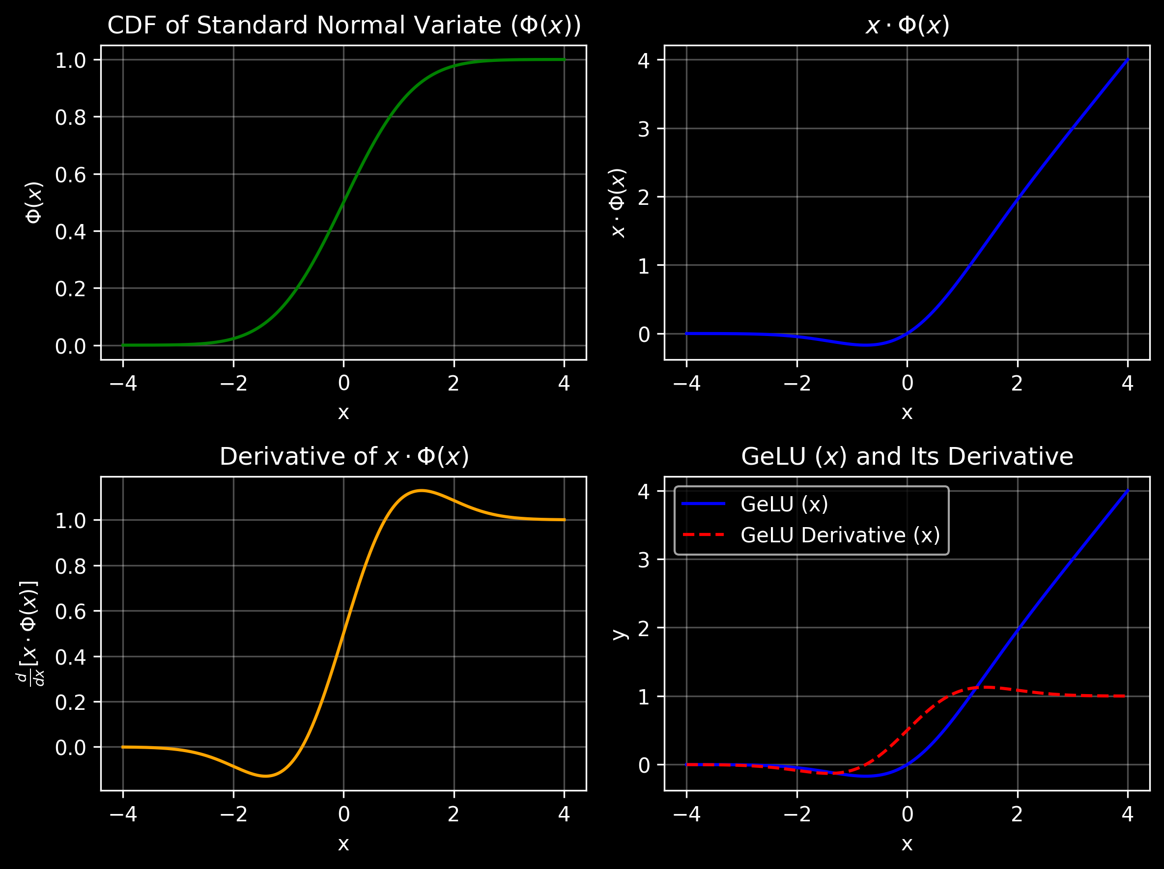
# Plot 1: CDF of Standard Normal Variate (Phi(x))
axs[0, 0].plot(x.detach().numpy(), phi_x.detach().numpy(), color='green')
axs[0, 0].set_title(r"CDF of Standard Normal Variate ($\Phi(x)$)")
axs[0, 0].set_xlabel("x")
axs[0, 0].set_ylabel(r"$\Phi(x)$")
axs[0, 0].grid(alpha=0.3)
# Plot 2: x * Phi(x)
axs[0, 1].plot(x.detach().numpy(), x_cdf.detach().numpy(), color='blue')
axs[0, 1].set_title(r"$x \cdot \Phi(x)$")
axs[0, 1].set_xlabel("x")
axs[0, 1].set_ylabel(r"$x \cdot \Phi(x)$")
axs[0, 1].grid(alpha=0.3)
# Plot 3: Derivative of x * Phi(x)
axs[1, 0].plot(x.detach().numpy(), x_cdf_derivative.detach().numpy(), color='orange')
axs[1, 0].set_title(r"Derivative of $x \cdot \Phi(x)$")
axs[1, 0].set_xlabel("x")
axs[1, 0].set_ylabel(r"$\frac{d}{dx} \left[ x \cdot \Phi(x) \right]$")
axs[1, 0].grid(alpha=0.3)
# Plot 4: GeLU and Its Derivative (using x_input)
axs[1, 1].plot(x_input.detach().numpy(), gelu_x.detach().numpy(), label="GeLU (x)", color='blue')
axs[1, 1].plot(x_input.detach().numpy(), gelu_x_derivative.detach().numpy(), label="GeLU Derivative (x)", color='red', linestyle='--')
axs[1, 1].set_title(r"GeLU ($x$) and Its Derivative")
axs[1, 1].set_xlabel("x")
axs[1, 1].set_ylabel("y")
axs[1, 1].legend()
axs[1, 1].grid(alpha=0.3)
# Adjust layout
plt.tight_layout()
plt.show()