Ideal Properties of a Latent Space

1. Compactness

• Lower-dimensional than the input space

• Retains essential data features without redundancy

• Efficient representation for downstream tasks

2. Structured Organization

• Preserves semantic relationships between data points

• Similar inputs map to nearby latent points

• Enables meaningful interpolation and neighborhood operations

3. Disentanglement

• Each dimension represents an independent factor of variation

• Changes in one factor don’t affect others

• Provides interpretable and controllable representations

4. Continuity

• Smooth transitions in latent space yield smooth data changes

• No abrupt jumps or discontinuities

• Supports stable generation and interpolation

5. Generative Capability

• Random sampling produces valid, realistic outputs

• Well-defined probability distribution over latent space

• No “holes” or invalid regions

6. Class Separation

• Different categories form distinct clusters

• Clear decision boundaries for classification

• Supports both supervised and unsupervised tasks

7. Feature Invariance

• Robust to irrelevant input variations

• Captures task-relevant features

• Filters out noise and nuisance factors

8. Latent Smoothness

• Small perturbations yield predictable changes

• Stable behavior under optimization

• Supports gradient-based manipulation

Why AutoEncoder Latent Space Falls Short

Structural Issues:

• No guarantee of semantic organization

• Similar inputs can map to distant latent points

• Arbitrary encoding without meaningful structure

Poor Generation:

• Sparse coverage of latent space

• “Holes” between valid encodings

• Unrealistic outputs when sampling randomly

Limited Disentanglement:

• No mechanism for factor separation

• Entangled representations

• Difficult to control individual features

Improved Variants:

1. Variational AutoEncoders (VAEs)

   • Enforces continuous latent space

   • Gaussian prior for proper sampling

   • Better generation capabilities

2. β-VAEs

   • Enhanced disentanglement

   • Controlled information bottleneck

   • Trade-off between reconstruction and independence

3. Adversarial AutoEncoders

   • GAN-like training for better distribution matching

   • More realistic generation

   • Improved latent space structure

import itertools

import torch
import numpy as np
import random
import matplotlib.pyplot as plt
import torch.nn as nn
import torch.optim as optim
from torch.utils.data import DataLoader
from torchvision import datasets, transforms

# Set seed for reproducibility
SEED = 47
torch.manual_seed(SEED)
np.random.seed(SEED)
random.seed(SEED)
plt.style.use('dark_background')

# Set device based on availability of Cuda
device = torch.device("cuda" if torch.cuda.is_available() else "cpu")
print(f"Using {device} backend.")

Using cuda backend.

# Define data transforms
transform = transforms.Compose([transforms.ToTensor()])

# Load datasets
train_dataset = datasets.MNIST(root='./data', train=True, download=True, transform=transform)
test_dataset = datasets.MNIST(root='./data', train=False, download=True, transform=transform)
train_loader = DataLoader(train_dataset, batch_size=256, shuffle=True)
test_loader = DataLoader(test_dataset, batch_size=256, shuffle=False)

# AutoEncoder Model
class AutoEncoder(nn.Module):
    def __init__(self):
        super().__init__()
        self.encoder = nn.Sequential(
            nn.Flatten(),
            nn.Linear(28 * 28, 128), nn.ReLU(),
            nn.Linear(128, 64), nn.ReLU(),
            nn.Linear(64, 2)  # Latent space
        )
        self.decoder = nn.Sequential(
            nn.Linear(2, 64), nn.ReLU(),
            nn.Linear(64, 128), nn.ReLU(),
            nn.Linear(128, 28 * 28)
        )

    def forward(self, x):
        z = self.encoder(x)
        return self.decoder(z), z

# Initialize model, loss, and optimizer
model = AutoEncoder().to(device)
criterion = nn.MSELoss()
optimizer = optim.Adam(model.parameters(), lr=0.001)
model

AutoEncoder(
  (encoder): Sequential(
    (0): Flatten(start_dim=1, end_dim=-1)
    (1): Linear(in_features=784, out_features=128, bias=True)
    (2): ReLU()
    (3): Linear(in_features=128, out_features=64, bias=True)
    (4): ReLU()
    (5): Linear(in_features=64, out_features=2, bias=True)
  )
  (decoder): Sequential(
    (0): Linear(in_features=2, out_features=64, bias=True)
    (1): ReLU()
    (2): Linear(in_features=64, out_features=128, bias=True)
    (3): ReLU()
    (4): Linear(in_features=128, out_features=784, bias=True)
  )
)

# Training Loop
epochs = 50
for epoch in range(epochs):
    model.train()
    train_loss = 0
    for images, _ in train_loader:
        images = images.to(device)
        reconstructed, _ = model(images)
        loss = criterion(reconstructed, images.view(-1, 28 * 28))
        optimizer.zero_grad()
        loss.backward()
        optimizer.step()
        train_loss += loss.item()
    print(f"Epoch {epoch+1}/{epochs}, Loss: {train_loss / len(train_loader):.4f}")

Epoch 1/50, Loss: 0.0583

Epoch 2/50, Loss: 0.0485

Epoch 3/50, Loss: 0.0461

Epoch 4/50, Loss: 0.0446

Epoch 5/50, Loss: 0.0436

Epoch 6/50, Loss: 0.0428

Epoch 7/50, Loss: 0.0422

Epoch 8/50, Loss: 0.0415

Epoch 9/50, Loss: 0.0410

Epoch 10/50, Loss: 0.0406

Epoch 11/50, Loss: 0.0403

Epoch 12/50, Loss: 0.0400

Epoch 13/50, Loss: 0.0397

Epoch 14/50, Loss: 0.0395

Epoch 15/50, Loss: 0.0393

Epoch 16/50, Loss: 0.0391

Epoch 17/50, Loss: 0.0389

Epoch 18/50, Loss: 0.0387

Epoch 19/50, Loss: 0.0386

Epoch 20/50, Loss: 0.0384

Epoch 21/50, Loss: 0.0383

Epoch 22/50, Loss: 0.0381

Epoch 23/50, Loss: 0.0382

Epoch 24/50, Loss: 0.0380

Epoch 25/50, Loss: 0.0378

Epoch 26/50, Loss: 0.0377

Epoch 27/50, Loss: 0.0376

Epoch 28/50, Loss: 0.0375

Epoch 29/50, Loss: 0.0374

Epoch 30/50, Loss: 0.0374

Epoch 31/50, Loss: 0.0373

Epoch 32/50, Loss: 0.0371

Epoch 33/50, Loss: 0.0371

Epoch 34/50, Loss: 0.0371

Epoch 35/50, Loss: 0.0370

Epoch 36/50, Loss: 0.0369

Epoch 37/50, Loss: 0.0368

Epoch 38/50, Loss: 0.0367

Epoch 39/50, Loss: 0.0367

Epoch 40/50, Loss: 0.0367

Epoch 41/50, Loss: 0.0367

Epoch 42/50, Loss: 0.0367

Epoch 43/50, Loss: 0.0365

Epoch 44/50, Loss: 0.0366

Epoch 45/50, Loss: 0.0365

Epoch 46/50, Loss: 0.0364

Epoch 47/50, Loss: 0.0364

Epoch 48/50, Loss: 0.0364

Epoch 49/50, Loss: 0.0363

Epoch 50/50, Loss: 0.0363

# Extract latent space
model.eval()
latent_space, labels = [], []
with torch.no_grad():
    for images, y in train_loader:
        images = images.to(device)
        _, z = model(images)
        latent_space.append(z.cpu().numpy())
        labels.append(y.numpy())
latent_space = np.concatenate(latent_space)
labels = np.concatenate(labels)

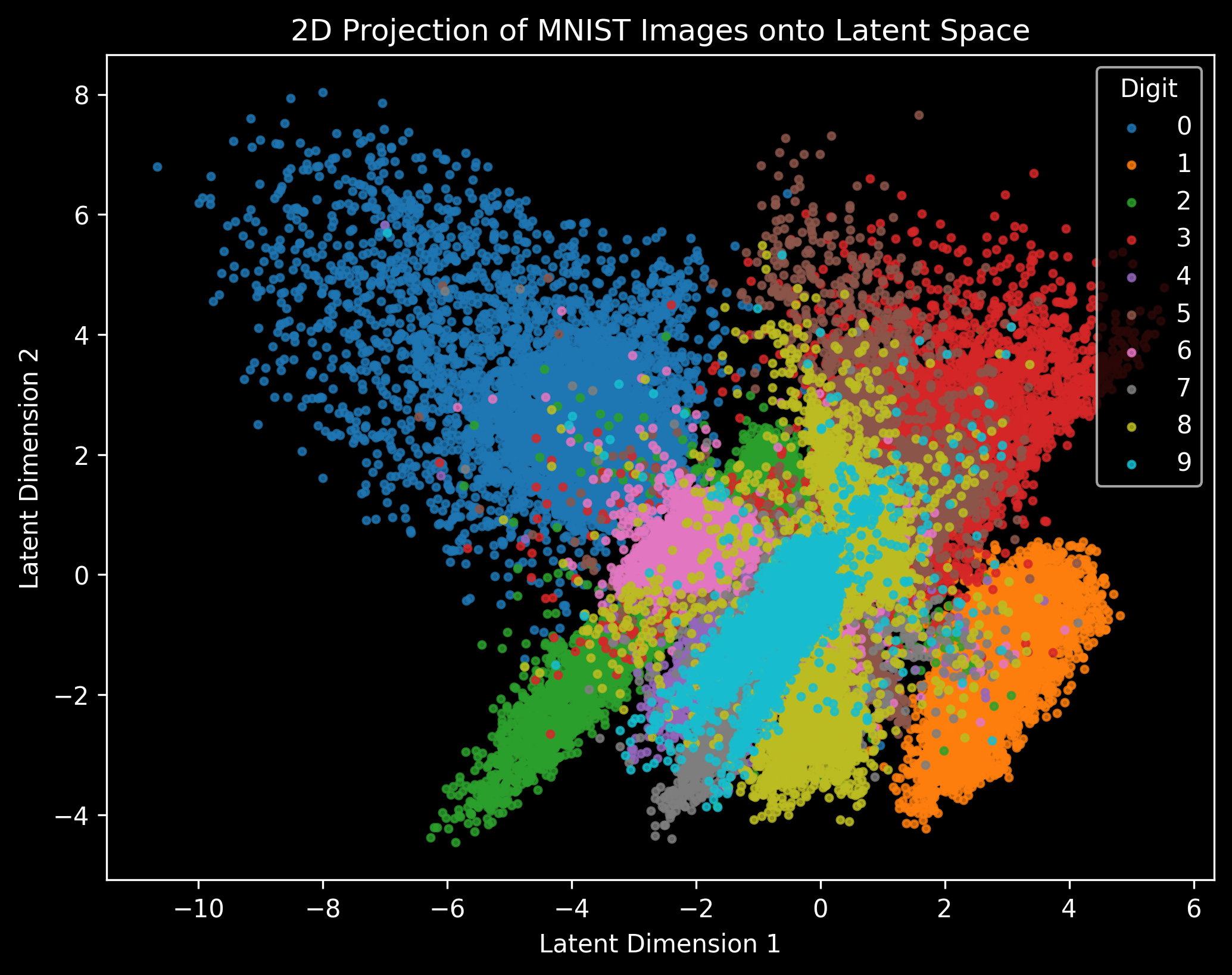
# Plot 2D Latent Space
plt.figure(figsize=(8, 6), dpi=300)
colors = ['#1f77b4', '#ff7f0e', '#2ca02c', '#d62728', '#9467bd', '#8c564b', '#e377c2', '#7f7f7f', '#bcbd22', '#17becf']
for class_label in range(10):
    indices = np.where(labels == class_label)
    plt.scatter(latent_space[indices, 0], latent_space[indices, 1], color=colors[class_label], label=str(class_label), alpha=0.8, s=8)
plt.legend(title="Digit", loc="upper right", fontsize=10)
plt.xlabel("Latent Dimension 1")
plt.ylabel("Latent Dimension 2")
plt.title("2D Projection of MNIST Images onto Latent Space")
plt.show()

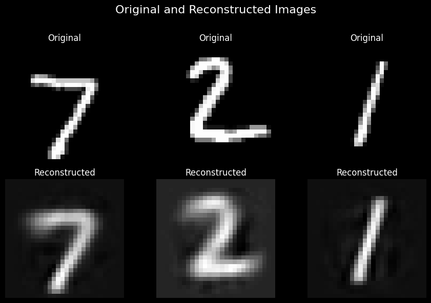
# Display Original and Reconstructed Images
def display_reconstructed_images(model, data_loader, num_samples=3):
    model.eval()
    fig, axes = plt.subplots(2, num_samples, figsize=(num_samples * 3, 6))
    fig.suptitle("Original and Reconstructed Images", fontsize=16)

    with torch.no_grad():
        for i, (images, _) in enumerate(data_loader):
            images = images[:num_samples].to(device)
            reconstructed, _ = model(images)
            
            for j in range(num_samples):
                axes[0, j].imshow(images[j].cpu().squeeze(), cmap='gray')
                axes[0, j].axis("off")
                axes[0, j].set_title("Original")
            
            reconstructed_images = reconstructed.view(-1, 28, 28)
            for j in range(num_samples):
                axes[1, j].imshow(reconstructed_images[j].cpu().squeeze(), cmap='gray')
                axes[1, j].axis("off")
                axes[1, j].set_title("Reconstructed")

            break
    plt.tight_layout()
    plt.subplots_adjust(top=0.85)
    plt.show()

display_reconstructed_images(model, 
                             test_loader, 
                             num_samples=3)

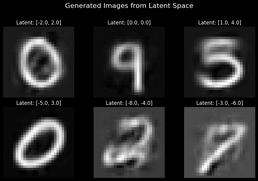
# Sample from Latent Space and Visualize
def sample_from_latent_space(model, latent_coords, grid_shape=(2, 3)):
    model.eval()
    latent_coords = torch.tensor(latent_coords, dtype=torch.float32, device=device)

    with torch.no_grad():
        generated_images = model.decoder(latent_coords).view(-1, 28, 28).cpu()

    fig, axes = plt.subplots(*grid_shape, figsize=(grid_shape[1] * 3, grid_shape[0] * 3))
    fig.suptitle("Generated Images from Latent Space", fontsize=16)
    axes = axes.flatten()

    for i, image in enumerate(generated_images):
        axes[i].imshow(image, cmap='gray')
        axes[i].axis("off")
        axes[i].set_title(f"Latent: {[round(x, 2) for x in latent_coords[i].tolist()]}")

    plt.tight_layout()
    plt.subplots_adjust(top=0.85)
    plt.show()

# Generate the arrays
latent_space_coords = [
    [-2, 2],
    [0, 0],
    [1, 4],
    [-5, 3],
    [-8, -4],
    [-3, -6]
]
sample_from_latent_space(model, 
                         latent_space_coords, 
                         grid_shape=(2, 3))